
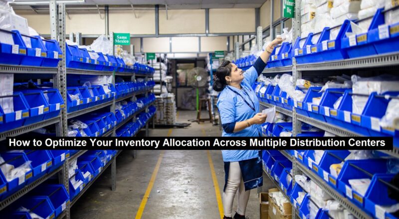
Most inventory teams do not struggle with allocation per se. The reason why they do struggle is that they do not trust their data, and allocation is the first place where it manifests. You will have a situation where for a particular SKU there is no stock in a warehouse while there is an excess in another, and the first thought that comes to your mind is that the forecast was wrong. It was not; the forecast was correct, but the barcode scan did not match the information in the ERP.
Stockouts and overstocks are the same problem with two faces
Not one single retailer intends to have an overstock of a certain SKU in one Distribution Center (DC) while being out of stock in another. Nevertheless, the situation occurs in almost every retail chain, since every allocation decision is made SKU/DC-specific without considering the entire network-wide supply-demand picture, resulting in a imbalanced network allocation which no one intended to create.
According to IHL research, inventory distortions (overstock and stockouts) cost global retailers over $1.1 trillion annually, with overstock representing the bigger portion of the losses in almost all retail chains. If the costs of overstock outweigh the revenues from additional sales, you are not buying too little; you are putting the inventory in the wrong place by misallocating it between your DCs, thus losing sales by not supplying the retail points of sale appropriately.
Fix the data before touching the allocation model
Before touching the allocation model think once more about the data integrity within your current system. If the barcode scans do not equal ERP data, stop there. Every allocation decision you make afterward will only perpetuate the same error on a larger scale and at a faster pace.
The objective of barcode scanning is to reconcile the physical inventory with the computerized one. Barcode scans should happen at every step of the logistics process: receiving, put-away, picking, packing, internal transfers, etc. If they only happen at one DC while other DCs record inventory manually at the end of the month, your cycle-counting efforts will be wasted on small discrepancies which will have a large impact on your network-wide allocation.
Cycle-counting efforts should also be ongoing throughout the year and not only during the annual “big count.” While 2% discrepancies across a handful of SKUs in several DCs may seem insignificant, having them network-wide means that the entire network makes allocation decisions based on incorrect data. Make data integrity your highest priority because everything else depends on it.
Read: How to Find a Tech Mentor and Get the Most Out of the Relationship
Segment SKUs before deciding on allocation rules
After you sync barcode scans and ERP data, the next most common mistake is to treat all SKUs the same way. Not every SKU should be in every DC, and not every SKU should be distributed across multiple DCs, as a significant amount of costs can be saved by optimizing DC-specific carrying costs.
High velocity-low variability SKUs and high velocity-high variability SKUs are great SKUs to consider for a wide distribution across multiple DCs because their demand can be forecasted with a high level of accuracy, and the benefits of proximity to the consumer outweigh the costs of inventory duplication.
Low velocity-high variability SKUs and low velocity-low variability SKUs should be considered for a tight distribution, ideally stored in one or a few DCs, because the costs of distribution across multiple DCs outweigh the benefits. It is often counterintuitive, but a SKU with a slow-moving velocity can still be a profitable SKU; however, its slow-moving nature dictates that it cannot be distributed widely without incurring additional costs from inventory duplication.
This distribution consideration is not static and should change with the SKU’s life cycle, velocity, and seasonality. An SKU that was great for a wide distribution in Q3 may turn out to be a poor candidate for it in Q1. Set a quarterly recurring process to review SKUs, their velocity, seasonality, and profile before making any distribution-wide changes.
Forecast at the DC level, not the network level
A lot of allocation challenges are born from the network-wide SKU forecast that gets split between the DCs according to a certain set of rules.
A SKU may have equal demand across all regions network-wide, but some DCs will ship more than others due to local demand, seasonality, and proximity to local consumers. If the demand spike only occurs in one region, the local DC will be out of stock while other DCs will have an overstock.
Forecasting at the DC level is more work but provides a more accurate baseline allocation for each DC. It is also critical to use historical sell-through data rather than raw units shipped, since the latter can be misleading if the previous allocation decisions were faulty.
Let replenishment lead time and transit cost to the consumer dictate how much you can thin your distribution
The longer the lead time (a period of time between when an order is placed and when it is received), the higher the local safety stock should be in a DC to account for the uncertainty of demand during that period. A DC with a longer lead time from the supplier will require a higher buffer than a DC with a shorter lead time.
The shorter the transit time to the consumer and the lower the cost of transportation, the more attractive it is to consolidate inventory in one DC rather than have it spread out across multiple DCs to serve different regions. The math of such a decision should be done individually for each DC to understand how extra days of supply for fast-moving SKUs can offset the costs and risks of adding another DC or using 3PL services.
This consideration in many ways defines the entire allocation strategy, and many retailers fail to do it correctly, resulting in too many DCs that are too close to the consumer but are costly to maintain with low inventory turnover.
Set safety stock with math, not a magic number
Using a magic number such as 20% for safety stock for every SKU across all DCs is not a great way to determine it. Some DCs will perform better than others based on historical sell-through data, and those that had a higher variance in sell-through should have a higher safety stock. This way, the DCs with consistent sales volumes throughout the year will not be penalized for the ones with lower volume but higher variance.
A more statistically accurate way to determine safety stock for each DC is to use the z-score that corresponds to the desired service level and multiply it by the standard deviation of demand during the lead time. The higher the variance and the longer the lead time, the higher the safety stock should be for that particular DC. It should be calculated for each DC/segment, and not across the entire network, since it will be different for each due to variance in sales and lead time.
While the calculation may seem tedious, it ultimately determines how much inventory is exposed to the risk of being written off as dead inventory in the DC, and it is crucial to prevent the two-headed problem of overstock in some DCs and understock in others.
Replenish per DC, not on a single company-wide clock
Many networks replenish on the same clock, meaning that every DC reorders on a weekly or biweekly basis or has a specific day of the week when the replenishment happens, regardless of their unique circumstances. While it may be easier to plan logistics and transportation this way, it is a poor practice to have all DCs operate on the same clock.
Every DC should have its own clock and should replenish based on its own unique sell-through performance, lead time, and safety stock requirements. A coastal DC handling fast-moving inventory may need to reorder every week or every few days, while an inland DC with a smaller population base may only need to reorder every couple of months. Using the same replenishment clock for both will create inevitable imbalances.
Once again, the integrity of the barcode scans plays a role here. The clock only works if the system that initiates the replenishment knows what the current stock level is at any given moment, not what it was during the last cycle-count.
Decide whether to build or rent capacity
As networks grow, they tend to seek to expand into new regions to meet the demand in those regions. The challenge that many networks face is that they have to make a difficult financial decision upfront to lease new warehouse space and hire staff to manage it while not knowing if the demand will be there to support it. This is where renting capacity from third-party logistics (3PL) providers makes more sense than building it in-house.
When a network rents capacity from a 3PL, it can position inventory closer to the consumer without committing to long-term leases or additional hires. It allows the network to serve a new region while still being able to scale up or down depending on the demand without having to invest in fixed assets. The only caveat is that the 3PL node should be integrated into the network in the same way as other DCs with near real-time barcode scans. If a 3PL operates on a different system with daily updates, it will recreate the same allocation challenges as if it were an independent DC, only at a greater scale. Use the same due diligence for a potential 3PL partner’s scanning and integration processes as you would for their square footage and dock availability.
Measure the right things and revisit the model
Allocation is an ongoing process and should be revisited periodically to ensure it still meets the performance requirements of the network. The most important metrics to measure are fill rate, inventory turnover, and days of supply at the DC level, and not the network level. A network fill rate or inventory turnover can be healthy while individual DCs are underperforming. Set a quarterly recurring process to review fill rates, inventory turnover, and days of supply at the DC level and optimize safety stock, reorder points, and DC-SKU allocations accordingly. Additionally, optimize DC-SKU allocations based on actual performance, and not theoretical models, to ensure you are capturing the value of proximity to the consumer for fast-moving SKUs while not overpaying for it for slow-moving SKUs.
The DCs that were ideal for your network 18 months ago may be ideal for somebody else’s network today. Make sure to revisit the allocation model and the performance of your network periodically to ensure you are using the right metrics to drive the right decisions.
Fix the data before you touch the allocation model. Segment your SKUs before you decide on any allocation rules. Forecast where the inventory will be sold, not how much of it will be sold. After that, the allocation math becomes simple and repeatable.